Tutorial
Prerequisities
DSDPy (scripts in src package) is written in Python3. The recommended way to install
all the packages needed in src is through Anaconda. For those who are familiar with
pip installation, note that the required packages can also be installed through standard
way, but the details are not included in this documentation.
Required Packages
PySB
PySB is a framework for building mathematical rule-based models of biochemical systems as Python programs. The installation command with Anaconda is:
conda install -c alubbock pysb
Numpy
Numpy is a fundamental package for scientific computing with Python. The installation command with Anaconda is:
conda install -c anaconda numpy
Networkx
Networkx is a Python package for the creation, manipulation, and study of the structure, dynamics, and functions of complex networks. This package is used in src for output incidence matrix. The installation command with Anaconda is:
conda install -c conda-forge networkx
Matplotlib
Matplotlib is a Python 2D plotting library, used in src for visualization of the simulation results. The installation command with Anaconda is:
conda install -c conda-forge matplotlib
PyQt
PyQt is a set of Python v2 and v3 bindings for The Qt Company’s Qt application framework and runs on all platforms supported by Qt including Windows, macOS, Linux, iOS and Android. The installation command with Anaconda is:
conda install -c anaconda pyqt
Bidict
Bidict is the bidirectional mapping library for Python. One can use one of the following commands to install:
conda install -c conda-forge bidict
conda install -c conda-forge/label/gcc7 bidict
conda install -c conda-forge/label/cf201901 bidict
conda install -c conda-forge/label/cf202003 bidict
Use
The core is a Python package (src) that includes scripts to run a DSD system analysis. One should be able to run the scripts if the required packages above have been downloaded.
DSDPy has a graphical user interface implemented as interface.py in the project root directory. To run this interface from command line interface, simply do:
python interface.py
Please make sure you have the Python package (src) in the same directory before you run the interface.
Programmatic Use
The entry point to the analysis of a DSD system is through [start_processor] function. To get test inputs for DSDPy, you need to download the res package (In the case you would like to make your own input, simply pass the file directory accordingly to function [start_processor] as suggested). After that, you can test if the DSDPy works by running the following command from a Python interpreter:
>>> from src import start_processor as sp
>>> sp.start_processor(filedir='./res/input')
RB: {(2, 0), (0, 3)}
R4: {(0, 2), (2, 1)}
R3: {(1, 0), (3, 1)}
RU: {(2, 0), (0, 3)}
R4: {(0, 2), (2, 1)}
R4: {(1, 1), (0, 2)}
R3: {(1, 0), (3, 1)}
RU: {(0, 1), (1, 2)}
R4: {(1, 1), (0, 2)}
RU: {(0, 1), (1, 2)}
R3: {(0, 0), (1, 1)}
RB: {(0, 1), (2, 2)}
RB: {(0, 1), (2, 2)}
Note: This test input is res/input.
Creating Your Own Input
The ideal way to generate the input to DSDPy is through a GUI interface which enables a quickstart for people with DSD systems to test. However, such interface is now under development and one needs to manually type the input for DSDPy.
An input for DSDPy needs at least three sections:
Species
Initial species of the DSD system in their canonical forms.
<> denotes a strand
// denotes seperation of species
^ denotes toehold
* denotes complementary
! denotes bonded, what follows is the bond name
The strands are parsed always from 5’-end to 3’-end.
An example format:
<L T2^!i2 X*!i1 T1^>
<A X!i1 T2^*!i2>
//
<T1^* X!j1 R>
<X*!j1 A*!j2>
<A!j2>
Information on Species
Names of the initial species (order corresponds to the order of species above) and their initial copies. An example format:
SomeName 1000
Kinetics
Rates of the reactions, includes 3-way migration, 4-way migration, binding and unbinding (R3, R4, RB and RU). An example format:
RB 1e6
RU 1.2
R3 78.12
R4 5.6e-3
Additionally, the input can include the following sections:
Output directory
The directory for output files. An example format:
../output
Simulation settings
Simulation time and time steps. An example format:
1000 100
Note that the sections are all seperated by –.
Example input1
<L T2^!i2 X*!i1 T1^>
<A X!i1 T2^*!i2>
//
<T1^* X!j1 R>
<X*!j1 A*!j2>
<A!j2>
--
ss1 1000
ss2 1000
--
RB 1e6
RU 1.2
R3 78.12
R4 5.6e-3
Example input2
<f1^ x!1>
<to^* x*!1>
//
<b!2 tx^!3>
<to^*!4 x*!5 tx^*!3 b*!2 tb^*>
<x!5 to^!4>
//
<tx^ x>
//
<tb^ b>
--
ss1 100
ss2 100
ss3 10
ss4 10
--
RB 1e6
RU 1.2
R3 78.12
R4 5.6e-3
--
../output
--
1000 100
Obtaining the Output
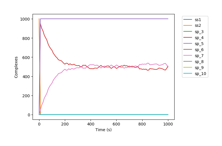
The output files includes a text file containing the information of the reaction network and a png file visualizing the BNG simulation results. These files can be found under the output directory or an user defined output directory.
Text File on the Reaction Network
The file contains three parts of information:
A species list that includes all the possible species in the network.
A reaction list that includes all the possible reactions in the network.
An incidence matrix based on the reaction network. (Its row denotes species and its column denotes the edge from one species to another)
Based on the example input1
-----Species-----
1
<L T2^!1 X*!2 T1^>
<A X!2 T2^*!1>

2
<T1^* X!1 R>
<X*!1 A*!2>
<A!2>

3
<L T2^!1 X*!2 T1^!3>
<A X!2 T2^*!1>
<T1^*!3 X!4 R>
<X*!4 A*!5>
<A!5>

4
<L T2^!1 X*!2 T1^!3>
<A!4 X!2 T2^*!1>
<T1^*!3 X!5 R>
<X*!5 A*!4>

5
<A>

6
<L T2^!1 X*!2 T1^!3>
<A X!4 T2^*!1>
<T1^*!3 X!2 R>
<X*!4 A*!5>
<A!5>

7
<L T2^!1 X*!2 T1^!3>
<A!4 X!5 T2^*!1>
<T1^*!3 X!2 R>
<X*!5 A*!4>

8
<L T2^ X*!1 T1^!2>
<T1^*!2 X!1 R>

9
<A X!1 T2^*>
<X*!1 A*!2>
<A!2>

10
<A!1 X!2 T2^*>
<X*!2 A*!1>

-----Reactions-----
RB 1 + 2 --> 3 rate=1000000.0

R3 3 --> 4 + 5 rate=78.12

R4 3 --> 6 rate=0.0056

RU 3 --> 1 + 2 rate=1.2

R4 4 --> 7 rate=0.0056

R3 6 --> 7 + 5 rate=78.12

RU 6 --> 8 + 9 rate=1.2

R4 7 --> 4 rate=0.0056

RU 7 --> 8 + 10 rate=1.2

RB 8 + 9 --> 6 rate=1000000.0

RB 8 + 10 --> 7 rate=1000000.0

-----Incidence Matrix-----
[1, 3] [2, 3] [3, 4] [3, 5] [3, 6] [3, 1] [3, 2] [4, 7] [6, 7] [6, 5] [6, 8] [6, 9] [7, 4] [7, 8] [7, 10] [8, 6] [9, 6] [8, 7] [10, 7]
  1 [[ 1.  0.  0.  0.  0. -1.  0.  0.  0.  0.  0.  0.  0.  0.  0.  0.  0.  0.  0.]]
  2 [[ 0.  1.  0.  0.  0.  0. -1.  0.  0.  0.  0.  0.  0.  0.  0.  0.  0.  0.  0.]]
  3 [[-1. -1.  1.  1.  1.  1.  1.  0.  0.  0.  0.  0.  0.  0.  0.  0.  0.  0.  0.]]
  4 [[ 0.  0. -1.  0.  0.  0.  0.  1.  0.  0.  0.  0. -1.  0.  0.  0.  0.  0.  0.]]
  5 [[ 0.  0.  0. -1.  0.  0.  0.  0.  0. -1.  0.  0.  0.  0.  0.  0.  0.  0.  0.]]
  6 [[ 0.  0.  0.  0. -1.  0.  0.  0.  1.  1.  1.  1.  0.  0.  0. -1.  0. -1.  0.]]
  7 [[ 0.  0.  0.  0.  0.  0.  0. -1. -1.  0.  0.  0.  1.  1.  1.  0. -1.  0. -1.]]
  8 [[ 0.  0.  0.  0.  0.  0.  0.  0.  0.  0. -1.  0.  0. -1.  0.  1.  1.  0.  0.]]
  9 [[ 0.  0.  0.  0.  0.  0.  0.  0.  0.  0.  0. -1.  0.  0.  0.  0.  0.  1.  0.]]
 10 [[ 0.  0.  0.  0.  0.  0.  0.  0.  0.  0.  0.  0.  0.  0. -1.  0.  0.  0.  1.]]
Modify the Documentation
The documentation uses reStructuredText. One can modify this documentation using command make html
under path doc .